Procedural 2D Clouds : A mathematical approach to nature
A deep dive into generating procedural clouds using maths, followed by some tips to make them appear volumetric.
One of the biggest mistakes I made while developing this shader was not considering the computational cost. This cost me 2 days in live-production and a huge headache, but everything worked out in the end!
Clouds are something that have fascinated me, you, and possibly everyone at one point in their life. Even though they appear 2D in the sky, they actually have a lot of volume and mass to them. This also means they are computationally heavy to render/generate. My target was to use something that was NOT a volume, and what else would work if not noise! I have a separate blog for different noises lined up, so keep out an eye ;)
In this breakdown, I’ll walk through a texture-based, optimized 2D cloud shader I wrote in Godot. It’s the system I developed for a recent project at Zitro, and it handles a huge amount of clouds while maintaining performance. The is not a “cool clouds” shader, rather performance-centric.
Non-Procedural Noise
The shader is built around a single-texture with multiple textures packed into different channels. If you are new to image processing, a typical image is usually comprised of RGB channels, usually
represented by JPEG. Often times there is a fourth one as well called Alpha, making the image RGBA, with the following extensions PNG, EXR, TARGA, TIFF. For this shader, the channels are as
follows:
- Red Channel (R): Static shape mask
- Green Channel (G): Tiled, primary scrollable noise
- Blue Channel (B): Tiled, secondary scrollable noise
Why?
Well, this way we avoid any expensive procedural noise functions and instead rely on texture lookups. These are almost always quicker, and since we have all the data in one image (AKA Texture), we only need one lookup and one load cycle. We can simply access the various channels/sub-textures using swizzling in GLSL (OpenGL Shading Language). This is a shorthand notation of extracting data from a container data type such as vec3.
void fragment() {
    vec4 tex = texture(TEXTURE, UV);

    // Getting red, green, blue channels
    vec3 tex_rgb = tex.rgb;

    // Getting individual channels
    float red = tex.r;
    float green = tex.g;
    float blue = tex.b;
}
You can grab the image below. The funky colours are due to different data present in each channel.
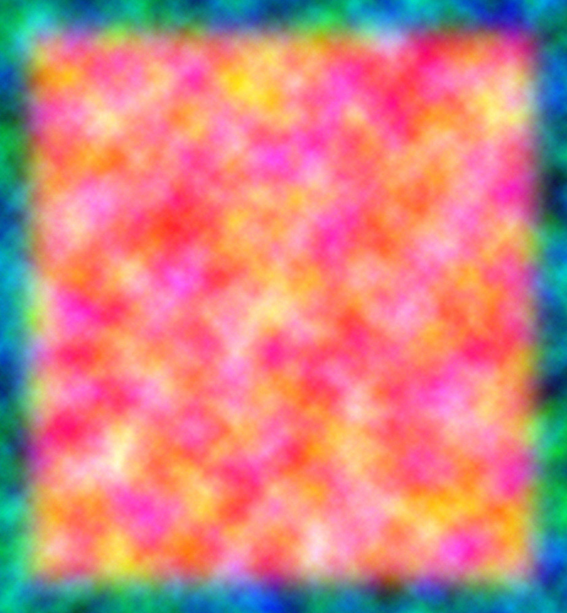

Red: Shape Mask

Green: Primary Noise

Blue: Secondary Noise
If you use Unreal Engine/Quixel, or any major asset shop, this is a very common technique to save texture lookups and memory. I got introduced to the concept a few years ago, and I haven’t been able to go back, it is truly the simplest optimization for any game.
Uniforms - Control Without Complexity
Alright, now we know how to sample a texture. But how do we pass it on to the GPU?
Uniforms!
Uniforms are special variables that act as a bridge between the CPU (Game Engine) and GPU (Shader). They are read-only parameters that remain constant across all vertices or fragments in a single draw call. Shaders run in parallel on thousands of pixels/vertices simulataneously. They cannot access you script variables directly as they are running on an entirely different processing environment, the GPU. Uniforms solve this by:
- Passing data once: You set a uniform value on the CPU, and every shader invocation sees the same value
- Staying constant: Unlike varying variables (which interpolate between vertices), uniforms don’t change during a single render pass
- Being efficient: One upload, many reads across all parallel threads
Common Use Cases
- Textures: Passing texture samplers (like our shape mask and noise textures)
- Colors: Theme colors, fog colors, etc.
- User settings & custom parameters: Slider values, toggle states
In our case, we’ll use a uniform to pass our noise texture and shape mask to the fragment shader, making it accessible for cloud generation. Another great thing about uniforms is that you can make changes after compilation. A simple comaprison for uniforms can be made with Material Instance in Unreal Engine. The shader is compiled once and you can have multiple variations for the same using uniforms. Analogous to polymorphism in Object Oriented Programming (OOPs).
UV & Motion Controls
// Uniforms
uniform vec2 uv_scale = vec2(100, 75);

// Wind control
uniform vec2 direction = vec2(1.0, 0.0);
uniform float cloud_scale = 1.5;
uniform float speed : hint_range(-1.0, 1.0) = 0.03;
These uniforms define the spatial scale and motion of the clouds.
uv_scale and cloud_scale is used to scale the UVs. This can cause stretching/squashing along with scaling, which is desired for clouds.
direction and speed together define wind movement. They have been separated for granular control over both aspect.
Lighting & Composition Controls
// Artistic Controls
uniform float cloud_dark = 0.5;
uniform float cloud_light = 0.3;
uniform float cloud_cover : hint_range(-10.0, 1.0) = 0.2;
uniform float cloud_alpha : hint_range(0.0, 3.0) = 0.25;
uniform float sky_tint : hint_range(0.0, 1.0) = 0.6;

// Sky Hue
uniform vec4 sky_colour_01 : hint_color = vec4(0.2, 0.4, 0.6, 1.0);
uniform vec4 sky_colour_02 : hint_color = vec4(1.0, 0.647, 0.0, 1.0);
These parameters are artist-friendly. As a technical artist and graphics engineer, it is my job to make these shaders/tools accessible to the artists. Parameters are a great way of doing so. I sat down with an artist and managed to get some incredible results based on their tweaking! The eye and experience of an artist should be respected more than it is nowadays.
Instead of physically-based lighting, I use simple scalar parameters to control various aspects of the cloud. This ensures smooth performance in real-time and avoids reworking noise functions or the shader.
Vertex Shader - Why It Exists Here?
The vertex shader runs only four-times for a quad, once per vertex. I am using a simple plane to render out the clouds for our project. This is helpful when
you look at the holistic picture. Our target resolution is native 2160 x 6000, sometimes even more. Considering I sample the noise texture multiple times,
an average of 15 per fragment, the total number of times I need to sample the texture would be:
2160 x 6000 = 12,960,000 (Total fragments)
12,960,000 x 15 = 194,400,000 (Texture Samples)
Phew! That is a VERY large number. Thanks to modern GPUs, these computations do not mean a lot, but if your target is mobile devices, or weaker hardware, this becomes a problem. Like it did for me, while using procedural noise (Oh yes, the count was almost 30x than this).
The vertex shader helps reduce some calculations that will remain constant throughout the lifetime of the shader.
// flat varying vec2 cloud_uv : No interpolation, use vertex A's value
varying vec2 cloud_uv;
varying vec2 time_vec;
varying float aspect_ratio;

void vertex() {
	aspect_ratio = (uv_scale.y != 0.0) ? (uv_scale.x / uv_scale.y) : 1.0;

	// Fix aspect ratio so clouds look consistent on different screen sizes
	cloud_uv = UV * vec2(aspect_ratio, 1.0) * cloud_scale;

	// TIME for animating the clouds
	time_vec = TIME * speed * direction;
}
Anything that doesn’t need per-pixel precision, such as aspect ratio or time-based offsets, is calculated here and passed down as varyings.
While this may look like an insignificant optimization, but in shaders that are rendered across large screens, these choices add up.
Understanding the varying keyword
The varying keyword is a bridge between vertex shader and fragment shader. It gets calculated once per vertex and then gets interpolated across the entire surface for every
fragment (pixel) that gets rendered. Consider the following code snipped:
// VERTEX SHADER (runs 4 times for a quad)
// Computes and send interpolated value to fragment shader
varying vec2 cloud_uv;

void vertex() {
    // This runs ONLY 4 times (once per corner of the quad)
    cloud_uv = UV * vec2(aspect_ratio, 1.0) * cloud_scale;
}

// FRAGMENT SHADER (runs millions of times)
varying vec2 cloud_uv;

void fragment() {
    // cloud_uv is automatically interpolated between the 4 vertex values
    // So every pixel gets a smoothly blended value
}
When the GPU processed a quad (rectangle):
-
Vertex Shader calculates
cloud_uvat each of the 4 vertices (corners)- Top-left corner: cloud_uv = (0.0, 1.0)
- Top-right corner: cloud_uv = (1.0, 1.0)
- Bottom-left: cloud_uv = (0.0, 0.0)
- Bottom-right: cloud_uv = (1.0, 0.0)
-
The GPU automatically interpolates these values across the surface
- A pixel in the center gets cloud_uv ≈ (0.5, 0.5)
- A pixel 25% from the left gets cloud_uv ≈ (0.25, y)
-
Fragment Shader receives the interpolated value for each pixel and runs the
void fragment()code on each pixel.
Having mentioned texture lookup and sampling multiple times, what do they actually mean?
Texture Lookup & Sampling
The act of fetching a particular pixel’s colour (texel) from a texture using UV coordinates. Instead of computing noise mathematically, the function samples noise directly from a texture channel (As shown above).
The green and blue channels provide two independent noise sources, which can be layered and animated separately. This keeps the shader fast and predictable across hardware. Why predictable? Each system’s RNG (Random Number Generator) will produce a different value, which may cause artifacts or broken textures. The code below is used to sample noise based on a parameter (channel).
float texture_noise(sampler2D tex, vec2 p, int channel) {
	if(channel == 0) {
		return texture(tex, p).g;
	} else {
		return texture(tex, p).b;
	}
}
Texture sampling is the process of using interpolated UV coordinates in the fragment shader to fetch texel values from a texture. A single texture lookup returns all channels (RGBA) so you can swizzle out the green and blue channels as independent noise sources for layering and animation. Swizzling is a shorthand in GLSL where you can access various channels in a container data-type by using:
vec3 pos = vec3(0.1, -10.3, 4.0);

// Extracting the X, Y, and Z channels and their combinations from a predefined vector
float a = pos.x; // The resultant value will be 0.1
vec2 b = pos.yx; // The resultant vector will be (-10.3, 0.1)
vec3 c = pos.zzy; // The resultant vector will be (4.0, 4.0, -10.3)
Swizzling provides you an easy way to grab different components of a data container (for example: color.rgb, pos.xy or pos.zzx), allowing concise access, reordering and replication of channels.
Fractal Brownian Motion (FMB)
Adding different iterations of noise (octaves), where we sample the noise at different scales, rotations, and decreasing amplitude. This way we get more granulatiry in the noise and get more fine detail. This technique is called **Fractal Browning Motion (fBM), or simply, fractal noise. The following code achieves the same:
// Rotation matrix for FBM layers
const mat2 m = mat2(vec2(1.6, 1.2), vec2(-1.2, 1.6));

float fbm(sampler2D tex, vec2 n, int channel) {
	float total = 0.0, amplitude = 0.1;
	for(int i=0; i < 4; i++) {
		total += texture_noise(tex, n, channel) * amplitude;
		n = m * n;
		amplitude *= 0.4;
	}
	return total;
}
Here m is a constant matrix, which helps break visible tiling while keeping the math minimal.
Animated Noise
This function builds animated noise by repeatedly samplign the texture while progressively altering UVs and weights. This function is the heart of the shader.
By exposing various parameters, the same function can be reused for:
- Cloud Shape
- Detail Breakup
- Colour Variation
For our use case, we have used a extracted the colours extracts from the sky. This is done in the void fragment() function. Below you can find the
noise animation function that I have used for generating the clouds:
// Optimized animation function using texture lookups
float animate_noise(sampler2D tex, int channel, vec2 time_offset, vec2 uv, float q, float uv_step, float weight, float weight_step, int steps) {
	float val = 0.0;
	vec2 uv2 = uv * uv_step - q + time_offset;

	for(int i = 0; i < steps; i++) {
		val += abs(weight * texture_noise(tex, uv2, channel));
		uv2 = m * uv2 + time_offset;
		weight *= weight_step;
	}

	return val;
}
Fragment Shader - Putting it All Together
Below is a detailed breakdown of the fragment shader used.
Masking
The red channel of our sampled texture defines a mask where the clouds are allowed to exist. This keeps the edges clean, smooth, and avoids procedural noise bleeding outside the intended shape.
float mask = texture(TEXTURE, UV).r;Using the shape is as simple as multiplying the alpha of the final image with this mask.
COLOR.a *= mask;This circumvents the need to write any edge blending logic and blurring/lowering opacity; at the cost of some memory. Below you can see the difference between having a mask and not. The left image (without mask) shows harsh edges and seams between textures. The right image (with mask) solves this issue, giving a much more natural result.

Without Mask

With Mask
Noise Construction
I first build a base FBM signal q, then layer ridged and smooth noise on top of it. By sampling different noise textures between each noise sample, it gives more natural,
randomized results, breaking tiling, and adding visual complexity.
// 0. Base FBM (Pass TEXTURE sampler)
float q = fbm(TEXTURE, cloud_uv * 0.5, 0);
Here, a low-frequency FBM noise at half the UV scale is generated. This is used to wrap/distort UV coordinates of subsequent noise layers, adding organic irregularity. The 0 means
it samples the green channel.
// 1. Ridged Noise Shape (Pass TEXTURE sampler)
float r = animate_noise(TEXTURE, 0, time_vec, cloud_uv, q, 1.0, 0.8, 0.7, 4);
This call generates the primary clouds shape using ridged noise (abs() in animate_noise). This means that the valleys become peaks, giving sharp clouds edges.
// 2. Noise Shape (Pass TEXTURE sampler)
float f = animate_noise(TEXTURE, 1, time_vec * 2.0, cloud_uv, q, 1.0, 0.7, 0.6, 4);

f *= r + f;
This function generated secondary detail noise that moves twice as fast, time_vec * 2.0. It samples the noise in the blue channel, and has a slightly softer falloff. I am then combining
both the noise layers non-linearly:
r + f= Ridged shape + detail noise.f *= (r + f)= Detail noise is amplified where clouds exist.
This creates denser detail in cloud areas and fade details in empty regions. It’s a cheap way to fake volumetri density, clouds look thicker and more detailed in their centers.
// 3. Noise Colour (Pass TEXTURE sampler)
float c = animate_noise(TEXTURE, 0, time_vec * 5.0, cloud_uv, q, 2.0, 0.4, 0.6, 3);
This generates a fast-moving, high-frequency noise for colour/brightness variation. This moved 5x faster than base clouds (time_vec * 5.0), creating a shimmer effect. This adds internal cloud lighing variation,
same parts darker, some brighter.
Each layer runs at a different speed and scale, which creates the illusion of depth and evolving volume.
Colour & Composition
The sky gradient is vertical and intentionally simple. The focus of the shader is motion and silhouette, not atmosphere scattering. I am pretty interested in this as well, maybe a future blog?!
The mix() function is used to generate a gradient, simply based on 2 uniform colours.
uniform vec4 sky_colour_01 : hint_color = vec4(0.2, 0.4, 0.6, 1.0);
uniform vec4 sky_colour_02 : hint_color = vec4(1.0, 0.647, 0.0, 1.0);

void fragment() {
    vec3 sky_colour = mix(sky_colour_02.rgb, sky_colour_01.rgb, UV.y);
}
Here UV.y = 0 is the bottom and render sky_colour_02; UV.y = 1, the top renders sky_colour_01. The mix() function linearly interpolates between them.
vec3 cloud_colour = vec3(1.1, 1.1, 0.9) * clamp((cloud_dark + cloud_light * c), 0.0, 1.0);Using the cloud_colour, I get subtle internal brightness variation. The uniforms defined on top control the look and feel for the same.
uniform float cloud_dark = 0.5;
uniform float cloud_light = 0.3;
uniform float cloud_cover : hint_range(-10.0, 1.0) = 0.2;
uniform float cloud_alpha : hint_range(0.0, 3.0) = 0.25;

void fragment() {
    f = cloud_cover + cloud_alpha * f * r;
}
I am recalculating the cloud density f. The calculations above control how much clouds exist at each pixel.
cloud_cover= Base amount of clouds (negative = less clouds).cloud_alpha * f * r= Shape noise × ridged noise, scaled by alpha.
float alpha = clamp(f + c, 0.0, 1.0);
vec3 result = mix(sky_colour, clamp(sky_tint * sky_colour + cloud_colour, 0.0, 1.0), alpha);
result gives us the final rgb colours for our clouds. This takes into accoun the sky’s colour. sky_tint controls the tint factor on the clouds. The final mix is done using the calculated alpha, which
is the cloud coverage mask. Wherever f + c is high, show clouds and vice versa.
Finally the end result is achieved by combining the resultant colour and alphas into a vec4.
COLOR = vec4(result, alpha * mask);Important Note!
This shader only renders the clouds and not the sky background. If you want to render the sky in the background as well, then you have to modify the final output to the following:
COLOR = vec4(result, mask);What this does is use the mask as the alpha. You can also use COLOR = vec4(result, 1.0), if you don’t want a soft falloff to the scene.
Optimization (Viewport Rendering, Upscaling)
This is by-far one of the most important section of this breakdown. Rendering at the local 2160 x 6000 resolution was causing a huge
performance drop. The solution? Very simple, and probably intuitive. In this age of AI and upscaling, we will use the same. I am using
Godot, which is an amazing open-source engine, for this task. The same concept can be used in any game engine using Render Targets.
Render Targets are Dynamic 2D Textures, whose content can be updated during runtime. They are useful for a bunch of things, for example,
a painting/drawing board in game. In Godot the hierarchy is as follows:
Godot Scene Hierarchy for Cloud Rendering
Here Node2D is the root of the scene, which acts as a container for all children node. In the texture rect I have created a ViewportTexture, which renders the Viewport node in a larger size. Godot
provides basic anti-aliasing algorithms such as FXAA, MSAA. This is a very basic method for upscaling and can be improved upon further with custom upscaling algorithms. One can create a custom node
with the required features. For my Clouds.tscn scene I have rendered the clouds in 3 layers with different properties and resolutions. The layers are as follows:
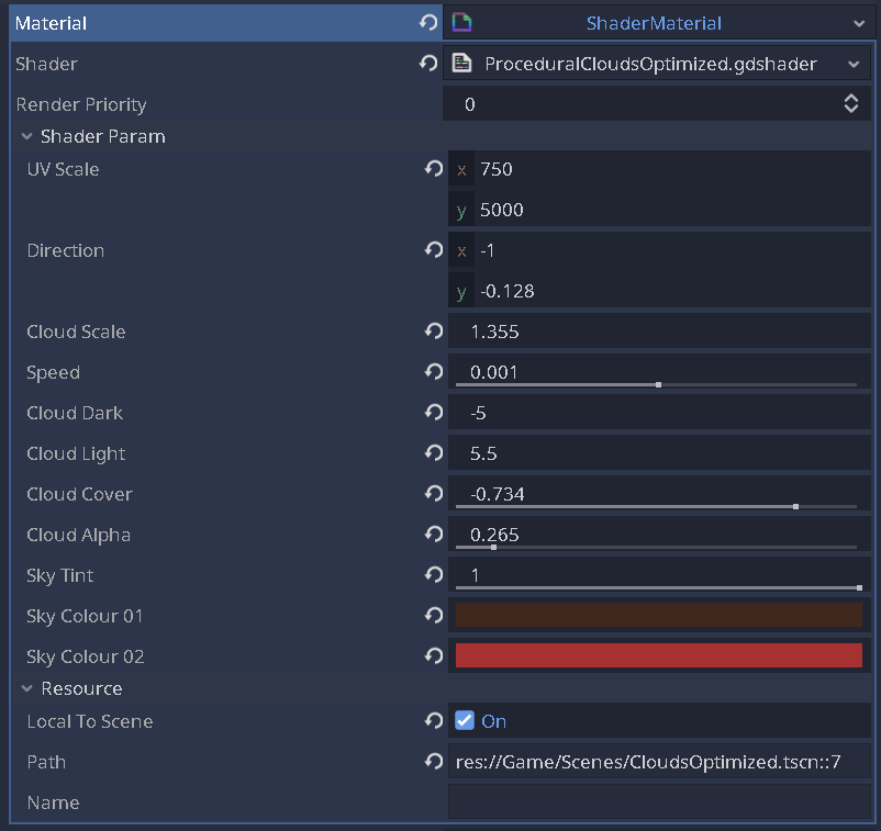
Horizon Clouds
These clouds are the farthest from the viewer’s perspective. I’ve squashed the rectangle so the clouds appear compressed, faking a horizon effect. The size of the rectangle is 558 × 200, which means:
558 × 200 = 111,600 pixels/fragments
With the optimized shader logic averaging ~15 texture samples per fragment (across FBM + animated noise layers), the total computation becomes:
111,600 × 15 = 1,674,000 texture samples
The settings I’ve used for colours, and other exposed parameters of the shader are given below. These settings completely depend on the artistic intent of the scene, so feel free to play around!
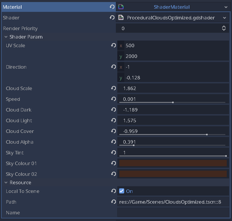
Middle Clouds
These clouds act as a middle-ground and move a bit faster than the background clouds to fake parallax. For this a rectangle of size 563 x 308 has been used. The clouds are slightly compressed.
563 x 308 = 173,404 pixels/fragments
173,404 x 15 = 2,601,060 texture samples
The shader parameters are given below:
Foreground Clouds
These clouds make up the main focal point of the scene, these clouds will have the most details visible. The are rendered across a rectangle of size 574 x 500
574 x 500 = 287,000 pixels/fragments
287,000 x 15 = 4,305,000 texture samples
These clouds have a lot of detail and move the fastest across the screen, giving a fake sense of depth. The shader parameters are given below:

Calculating the total samples based on the above calculations, we get:
4,305,000 + 2,601,060 + 1,674,000 = 8,580,060 samples
This is dramatically lower than rendering at full 2160 × 6000 resolution, which would require 194,400,000 samples. The loss in quality is also barely visible! Ingenious right? A simple trick can save
your butt at times of crunch.
Closing Section
The shader is not about realism, it’s about control, performance, and readability.
By relying on texture-packed noise and pushing work into the vertex stage, the shader stays lightweight while remanining visually flexible.
This approach works especially well for 2D skies, parallax backgrounds, and UI-driven scenes where full volumetric clouds would be un-necessary overhead.
Have questions about this approach? Find me on Twitter or shoot me an email :)